library(mypkgr)
library(devtools)
#> Loading required package: usethis
devtools::install_github("Florian-40/microbenchmark")
#> Using github PAT from envvar GITHUB_PAT
#> Downloading GitHub repo Florian-40/microbenchmark@HEAD
#> * checking for file ‘/tmp/Rtmp3hJpKq/remotes3546611b49d0/Florian-40-microbenchmark-c9b47c1/DESCRIPTION’ ... OK
#> * preparing ‘microbenchmark’:
#> * checking DESCRIPTION meta-information ... OK
#> * cleaning src
#> * running ‘cleanup’
#> * checking for LF line-endings in source and make files and shell scripts
#> * checking for empty or unneeded directories
#> * building ‘microbenchmark_1.4.9.tar.gz’
#> Installing package into '/home/runner/work/_temp/Library'
#> (as 'lib' is unspecified)
library(microbenchmark)
library(ggplot2)
Comparison with our microbenchmark package.
You can find microbenchmark package on my Git-Hub page : https://github.com/Florian-40/microbenchmark.git
mb <- microbenchmark(mvtnorm::dmvnorm(rep(1.96, 2)),
                     mvnpdf(x=matrix(rep(1.96,2)), Log=FALSE),
                     times=1000L)

mb
#> Unit: microseconds
#>                                           expr  min    lq     mean median    uq
#>                 mvtnorm::dmvnorm(rep(1.96, 2)) 63.2 73.20 103.0773   80.0 88.35
#>  mvnpdf(x = matrix(rep(1.96, 2)), Log = FALSE) 55.2 65.65  76.8534   70.9 78.25
#>      max neval
#>  20613.7  1000
#>   1702.4  1000
expression<-c('dmvnorm', 'mvnpdf')
autoplot(mb, expression)
#> Scale for 'y' is already present. Adding another scale for 'y', which will
#> replace the existing scale.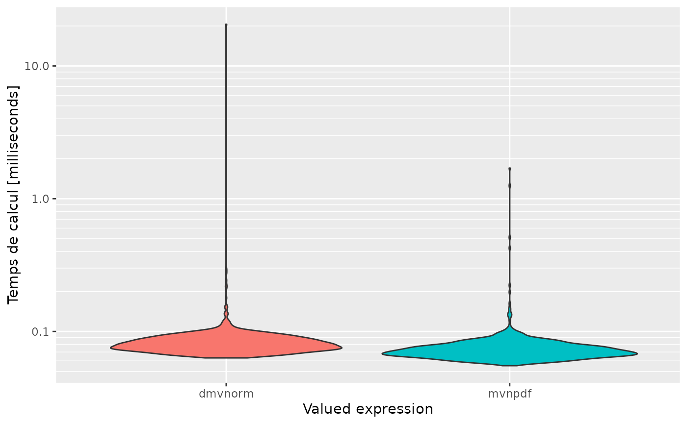
And with multidimensionnal, we get :
n <- 100
mb <- microbenchmark(mvtnorm::dmvnorm(matrix(1.96, nrow = n, ncol = 2)),
                     mvnpdf(x=matrix(1.96, nrow = 2, ncol = n), Log=FALSE),
                     times=100L)
mb
#> Unit: microseconds
#>                                                       expr   min     lq    mean
#>         mvtnorm::dmvnorm(matrix(1.96, nrow = n, ncol = 2))  73.3  80.65  93.405
#>  mvnpdf(x = matrix(1.96, nrow = 2, ncol = n), Log = FALSE) 621.5 648.10 698.946
#>  median     uq    max neval
#>    87.4  95.10  280.2   100
#>   669.3 703.55 2615.9   100
expression<-c('dmvnorm', 'mvnpdf')
autoplot(mb, expression)
#> Scale for 'y' is already present. Adding another scale for 'y', which will
#> replace the existing scale.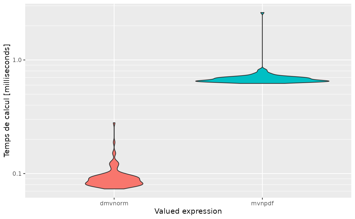
Profiling
By using this lines in terminal, we can check profiling of the code :
profvis::profvis({
+ n <- 10e4
+ pdfval <- mvnpdf(x=matrix(1.96, nrow = 2, ncol = n), Log=FALSE)
+ })
mvnpdfsmartfunction.
We can use new function mvnpdfmart and check profile with similar code :
profvis::profvis({
+ n <- 10e4
+ pdfval <- mvnpdfsmart(x=matrix(1.96, nrow = 2, ncol = n), Log=FALSE)
+ })
We can compare results with a microbenchmark :
n <- 1000
mb <- microbenchmark(mvtnorm::dmvnorm(matrix(1.96, nrow = n, ncol = 2)),
                     mvnpdf(x=matrix(1.96, nrow = 2, ncol = n), Log=FALSE),
                     mvnpdfsmart(x=matrix(1.96, nrow = 2, ncol = n), Log=FALSE),
                     times=100L)
mb
#> Unit: microseconds
#>                                                            expr    min      lq
#>              mvtnorm::dmvnorm(matrix(1.96, nrow = n, ncol = 2))  114.1  131.90
#>       mvnpdf(x = matrix(1.96, nrow = 2, ncol = n), Log = FALSE) 8038.3 8579.25
#>  mvnpdfsmart(x = matrix(1.96, nrow = 2, ncol = n), Log = FALSE) 5000.6 5454.35
#>      mean  median      uq     max neval
#>   194.642  181.55  216.75  1121.8   100
#>  9402.443 8794.65 9172.20 18258.9   100
#>  6368.446 5605.20 5947.00 13936.6   100
expression<-c('dmvnorm', 'mvnpdf', 'mvnpdfsmart')
autoplot(mb, expression)
#> Scale for 'y' is already present. Adding another scale for 'y', which will
#> replace the existing scale.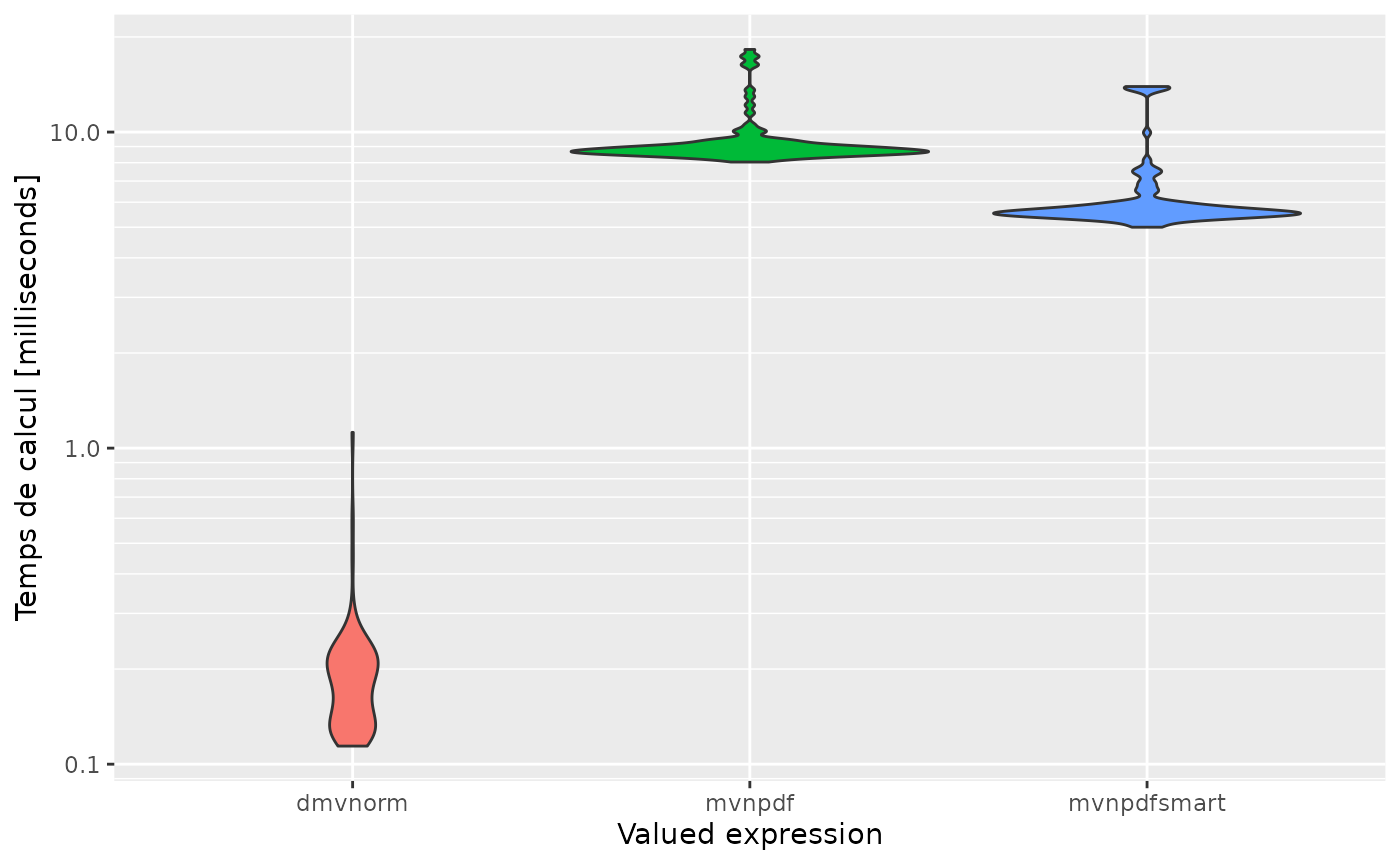
mvnpdfoptim function.
We can use new function mvnpdfmart and check profile with similar code :
profvis::profvis({
+ n <- 10e4
+ pdfval <- mvnpdfoptim(x=matrix(1.96, nrow = 2, ncol = n), Log=FALSE)
+ })
We can compare all results with a microbenchmark:
n <- 1000
mb <- microbenchmark(mvtnorm::dmvnorm(matrix(1.96, nrow = n, ncol = 2)),
                     mvnpdf(x=matrix(1.96, nrow = 2, ncol = n), Log=FALSE),
                     mvnpdfsmart(x=matrix(1.96, nrow = 2, ncol = n), Log=FALSE),
                     mvnpdfoptim(x=matrix(1.96, nrow = 2, ncol = n), Log=FALSE),
                     times=100L)
mb
#> Unit: microseconds
#>                                                            expr    min      lq
#>              mvtnorm::dmvnorm(matrix(1.96, nrow = n, ncol = 2))  111.4  137.90
#>       mvnpdf(x = matrix(1.96, nrow = 2, ncol = n), Log = FALSE) 8041.4 8404.85
#>  mvnpdfsmart(x = matrix(1.96, nrow = 2, ncol = n), Log = FALSE) 5107.1 5358.30
#>  mvnpdfoptim(x = matrix(1.96, nrow = 2, ncol = n), Log = FALSE) 3899.5 4129.80
#>      mean  median      uq      max neval
#>   176.643  180.00  204.20    362.3   100
#>  9205.713 8677.70 9090.40  16785.4   100
#>  7078.850 5529.45 5848.95 128585.3   100
#>  4897.239 4256.00 4450.10  15084.7   100
expression<-c('dmvnorm', 'mvnpdf', 'mvnpdfsmart', 'mvnpdfoptim')
autoplot(mb, expression)
#> Scale for 'y' is already present. Adding another scale for 'y', which will
#> replace the existing scale.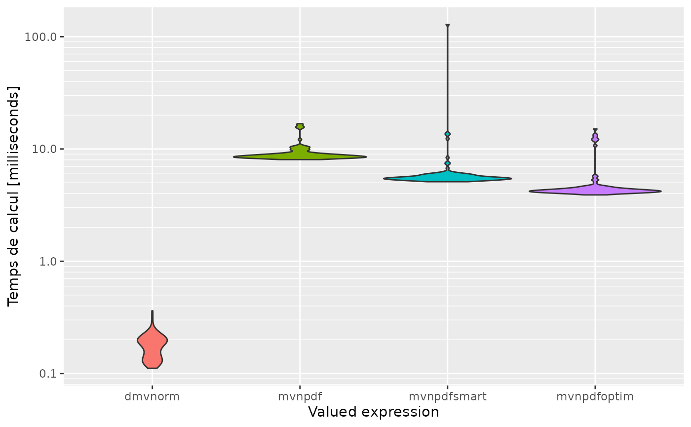
Using Rccp Armadillo functions.
We write a better inversion matrix with C++ language and we include it in mvnpdfsmart. Thus, we get microbenchmark :
n <- 1000
mb <- microbenchmark(mvtnorm::dmvnorm(matrix(1.96, nrow = n, ncol = 2)),
                     mvnpdf(x=matrix(1.96, nrow = 2, ncol = n), Log=FALSE),
                     mvnpdfsmart(x=matrix(1.96, nrow = 2, ncol = n), Log=FALSE),
                     mvnpdfoptim(x=matrix(1.96, nrow = 2, ncol = n), Log=FALSE),
                     mvnpdf_invC(x=matrix(1.96, nrow = 2, ncol = n), Log=FALSE),
                     times=100L)
mb
#> Unit: microseconds
#>                                                            expr    min      lq
#>              mvtnorm::dmvnorm(matrix(1.96, nrow = n, ncol = 2))  112.8  167.55
#>       mvnpdf(x = matrix(1.96, nrow = 2, ncol = n), Log = FALSE) 8070.7 8492.50
#>  mvnpdfsmart(x = matrix(1.96, nrow = 2, ncol = n), Log = FALSE) 4999.0 5484.55
#>  mvnpdfoptim(x = matrix(1.96, nrow = 2, ncol = n), Log = FALSE) 3953.4 4227.70
#>  mvnpdf_invC(x = matrix(1.96, nrow = 2, ncol = n), Log = FALSE) 5114.1 5451.15
#>      mean  median      uq     max neval
#>   198.911  194.95  216.70   447.1   100
#>  9103.868 8680.05 9076.45 15987.4   100
#>  6334.742 5659.85 5831.35 16775.6   100
#>  4991.840 4363.20 4561.55 14333.4   100
#>  6093.486 5613.50 5885.15 13621.8   100
expression<-c('dmvnorm', 'mvnpdf', 'mvnpdfsmart', 'mvnpdfoptim', 'mvnpdf_invC')
autoplot(mb, expression)
#> Scale for 'y' is already present. Adding another scale for 'y', which will
#> replace the existing scale.
Now, use complete implementation of mvnpdfsmart in C++.
Rcpp::sourceCpp("../src/mvnpdfC.cpp")
n <- 1000
mb <- microbenchmark(mvtnorm::dmvnorm(matrix(1.96, nrow = n, ncol = 2)),
                     mvnpdf(x=matrix(1.96, nrow = 2, ncol = n), Log=FALSE),
                     mvnpdfsmart(x=matrix(1.96, nrow = 2, ncol = n), Log=FALSE),
                     mvnpdfoptim(x=matrix(1.96, nrow = 2, ncol = n), Log=FALSE),
                     mvnpdf_invC(x=matrix(1.96, nrow = 2, ncol = n), Log=FALSE),
                     mvnpdfC(x=matrix(1.96, nrow = 2, ncol = n), mean = rep(0, 2), varcovM = diag(2), Log=FALSE),
                     times=100L)
mb
#> Unit: microseconds
#>                                                                                                  expr
#>                                                    mvtnorm::dmvnorm(matrix(1.96, nrow = n, ncol = 2))
#>                                             mvnpdf(x = matrix(1.96, nrow = 2, ncol = n), Log = FALSE)
#>                                        mvnpdfsmart(x = matrix(1.96, nrow = 2, ncol = n), Log = FALSE)
#>                                        mvnpdfoptim(x = matrix(1.96, nrow = 2, ncol = n), Log = FALSE)
#>                                        mvnpdf_invC(x = matrix(1.96, nrow = 2, ncol = n), Log = FALSE)
#>  mvnpdfC(x = matrix(1.96, nrow = 2, ncol = n), mean = rep(0, 2),      varcovM = diag(2), Log = FALSE)
#>     min      lq     mean  median      uq     max neval
#>   117.1  152.70  194.936  186.50  215.75   650.4   100
#>  7627.2 8397.55 9708.536 8835.15 9654.10 23144.3   100
#>  4850.3 5308.05 6247.285 5613.60 5892.25 18052.2   100
#>  3662.5 4161.70 4707.005 4338.95 4582.35 13037.8   100
#>  4775.4 5292.55 6129.456 5616.85 5883.90 14594.2   100
#>    48.4   63.10   96.326   72.75   84.90  1552.9   100
expression<-c('dmvnorm', 'mvnpdf', 'mvnpdfsmart', 'mvnpdfoptim', 'mvnpdf_invC', 'mvnpdfC')
autoplot(mb, expression)
#> Scale for 'y' is already present. Adding another scale for 'y', which will
#> replace the existing scale.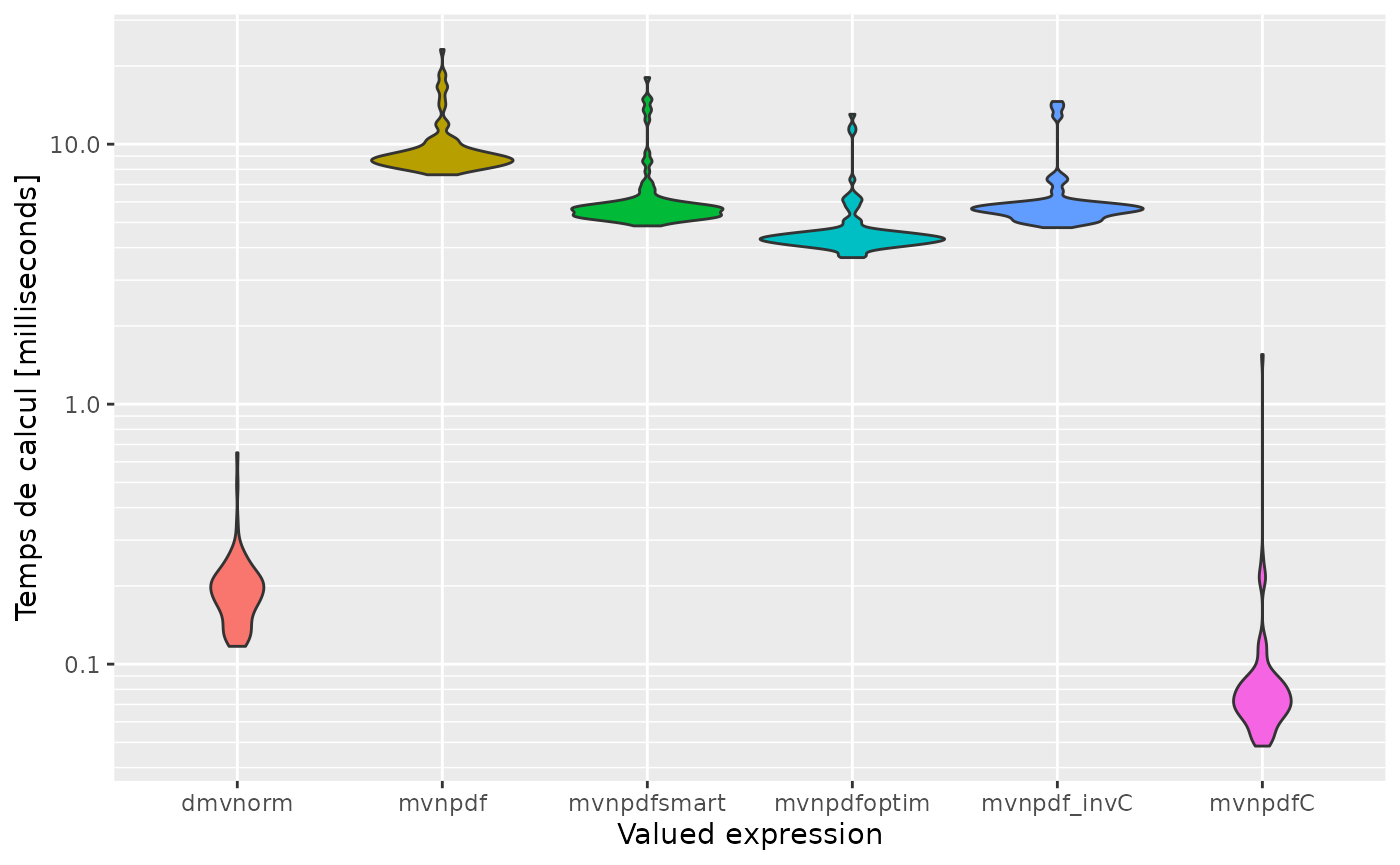
Parallel code
1st simple example.
Let’s try to calculate the logarithm of \(n\) numbers.
mb <- microbenchmark(log_par(1:100), log_seq(1:100), times=50)
mb
#> Unit: microseconds
#>            expr      min       lq       mean   median       uq      max neval
#>  log_par(1:100) 382460.3 411480.4 421754.696 418697.8 430139.0 468788.9    50
#>  log_seq(1:100)      2.2      2.8     17.208     10.8     12.7    351.4    50
expression <- c('log_par', 'log_seq')
autoplot(mb, expression)
#> Scale for 'y' is already present. Adding another scale for 'y', which will
#> replace the existing scale.